Tackling Numerical Difficulties in Linear Programming: What Every Modeler Should Know

Introduction

Linear programming (LP) is a go-to method for solving optimization problems in everything from supply chains to finance. But even the most elegant LP models can run into trouble—not because of logic errors, but due to numerical difficulties that creep in during computation.

Let’s explore what these issues are, why they happen, and how you can avoid them.

---

What Are Numerical Difficulties?

Numerical difficulties arise when the math behind your LP model becomes unstable or inaccurate due to the way computers handle numbers—especially floating-point arithmetic. These issues can lead to:

• Slow performance
• Incorrect solutions
• Solver crashes
• Misleading feasibility or optimality reports

---

Common Culprits (with Real-World Examples)

1. Ill-Conditioned Matrices

When your constraint matrix has values that vary wildly in magnitude, solvers can struggle.

Example: A harvest scheduling model with volumes in board-feet and individual areas smaller than 1/10th acre might include coefficients ranging from ${10}^{-6}$10−6 to ${10}^6$106 (or worse! I've seen it). This can cause the solver to miscalculate dual values or even fail to converge.

Harvest scheduling models typically represent large areas of land (thousands or even millions of acres). Stand volumes are similarly often hundreds of units per acre, along with prices that are also usually hundreds of dollars per unit. Multiplying these things together, it is possible to have objective function values in the hundreds of millions of dollars (greatly exceeding the 

$10^{-4}$ to ${10}^6$104 range that many solvers recommend). If your unscaled objective function is in the range of 100 million to 1 billion, you can always divide the outputs used in the objective function by 1,000,000 to get coefficients within the desired range.

---

2. Floating-Point Precision Errors

Computers can’t represent every number exactly, especially decimals. This leads to rounding errors.

Example: A constraint like $x+y=1$x+y=1 might yield $x=0.999999999$x=0.999999999, $y=0.000000001$y=0.000000001. Technically correct, but practically problematic—especially if your application requires clean, interpretable results. As a result, you should typically carry as many decimal places as possible, particularly in coefficients like area. For example, instead of an area record with 504.1, use 504.09775354.

---

3. Degeneracy

Degeneracy occurs when multiple basic feasible solutions exist at the same vertex. This can slow down or confuse the solver.

Example: In a network flow model (i.e., roads), several paths might have the same cost. The simplex method could cycle or take many iterations to find the optimal solution. Reprocess the network to eliminate redundancies by applying a shortest path algorithm.

---

4. Scaling Issues

When variables or constraints differ by several orders of magnitude, solvers may make poor pivoting decisions.

Example: One constraint is $0.0001x+0.0002y\le 1$0.0001x+0.0002y≤1, another is $1000x+2000y\le 5000$1000x+2000y≤5000. The solver might misinterpret the importance of each constraint due to the scale difference. A simple fix is to manually scale the constraints to be within the desired range 

$(10^{-4}$ to ${10}^6$104) by multiplying both sides of the inequality: $0.0001x+0.0002y\le 1$x+ y≤10000, x+ y≤5.

---

5. Infeasibility and Unboundedness Confusion

Sometimes, numerical noise makes it hard to tell if a model is truly infeasible or unbounded.

Example: Nearly parallel constraints might appear to intersect due to rounding, leading the solver to falsely report feasibility. These ones may be difficult to spot. As always, if you start experiencing infeasibility or difficulties solving, consider backtracking by removing constraints and then adding them back in one at a time to see which one(s) cause(s) problems.

---

How to Fix or Avoid These Issues

Here are some practical tips:

• Normalize Your Model: Keep coefficients within a similar range. Avoid extreme values.
• Validate Results: After solving, double-check constraint satisfaction and objective values—especially in critical applications.
• Use Solver Preprocessing: Most solvers offer automatic scaling and presolve routines. However, they can't necessarily fix every scaling problem.
• Adjust Tolerances: Unless you know what you're doing, you are better off leaving default tolerances alone. However, sometimes an adjustment can fine-tune feasibility and optimality tolerances to reduce rounding errors. Consult your server's online help and documentation.
  

---

Final Thoughts

Numerical difficulties in LP models are often overlooked but can have serious consequences. By understanding the root causes and applying smart modeling practices, you can build more robust, reliable optimization models.

Have you run into any of these issues in your own work? Let’s talk about it in the comments!

A New Open-Source Solver

Introduction

Most Woodstock users are probably running MOSEK as their default LP solver. As commercial software, it offers fast performance on standard LP formulations, it is relatively inexpensive, and it is supported by Remsoft directly. However, if your models include all-or-nothing decisions like *CUTCOMPLETECLASS, adjacency, or roading, MOSEK is not the best choice. This is not a fault of MOSEK -- it was designed to be a fast LP solver -- but its performance lags behind solvers like Gurobi or CPLEX. Gurobi and CPLEX are very good at solving mixed-integer programs (MIPs) but they are very expensive.

Of the open-source solvers supported by Remsoft, the COIN-OR solver CBC probably offers the best performance. However, I've noticed that finding up to date precompiled binaries of CBC that actually work with Woodstock can be difficult. The most recent version I could find is 2.10.11, compiled with MS Visual C 17. It works, but the performance on even some large LP only problems is not terribly good.

Recently, I read about a new open-source solver initiative called HiGHS: open source serial and parallel solvers for large-scalesparse linear programming (LP),mixed-integer programming (MIP), and quadratic programming (QP) models. My initial testing on some existing MPS files generated from Woodstock MIP models showed very good performance. However, reading and solving an MPS file doesn't help very much when you require a SCHEDULE file to create reports and graphs. Luckily, the HiGHS solver can take a parameter file like MOSEK or Gurobi, and in there you can specify one of 5 solution file output formats. Luckily, two of the options copy the format of the GLPSOL solver (Remsoft defines it as GNU). When I created a new MPS file and solved it with the GLPSOL solution format, I was able use Woodstock's LP2WK.exe converter to create a SCHEDULE file.

Steps To Make It Work

Setting Up HiGHS (workaround)

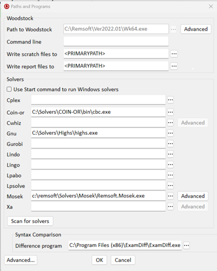
1. Download the HiGHS solver and save the executable in a subdirectory (e.g., C:\Solvers\HiGHS\highs.exe). In Woodstock, use Tools|Paths & programs to point to highs.exe in the GNU choice.
2. Create a text file called highs.par. Include the following line of code to specify the solution file format (GLPSOL): write_solution_style=3. If you're solving a MIP formulation, options like heuristics (%) and gap% are useful: mip_heuristic_effort=0.3 mip_rel_gap=0.001 
3. In Woodstock, specify *FORMAT GNU in the OPTIMIZE section. 
4. Press F9 to generate the matrix and create the batch file. You need to edit the batch file that Woodstock creates to comply with HiGHS command line parameters similar to below: C:\Solvers\Highs\highs.exe --model_file "model.mps" --solution_file "model.prt" --options_file highs.par
5. Use the Run|Run model.bat file menu or press F7 to call the solver and write the SCHEDULE section.

A Quirk of the HiGHS Solver

Although the programmable interfaces to HiGHS allow you to change the objective sense (MAX vs MIN), I didn't find any options in the command line interface to allow anything other than minimization. However, this is not a real problem because a MAX problem can be converted to a MIN problem by simply multiplying the outputs by -1. For example, the line 

            _MAX ordTOT - ocdLOG - ocdPLT 1..._LENGTH

can be converted to the equivalent statement 

           

            _MIN ocdLOG + ocdPLT - ordTOT 1.._LENGTH

Summary

If you are not running MIP formulations and you have MOSEK, there's nothing to see here folks. MOSEK is a very capable LP solver. Similarly, if you have access to Gurobi or CPLEX through school or corporate licensing, HiGHS is not going to be compelling. However, if you're interested in trying out some MIP formulations without investing a ton of money into a solver like Gurobi or CPLEX, give HiGHS a try. I'm hoping that Remsoft will soon support this new solver so that we don't have to do this messing around with batch files, etc. However, it is a small price to pay for a capable solver even now.

Don't hesitate to contact me if you have questions about this or other modeling topics!