Improve Model Efficiency - Part 1

Introduction

Someone once asked me, “When someone asks you to look at their model and make suggestions, what do you look for?” I thought this might be a good topic for a series of blog posts on modeling best practices to make QA easier.

The first thing I ask a client is what prompted the request? Is the model running too slow? Does it take a long time to solve? Does the solver struggle with feasibility? In most cases, the usual answer is, “it takes a long time to generate and solve.” That starts me thinking about efficiency in terms of development types and decision variables. Cardinal rule #1: avoid code that is difficult to understand or hides meaning.

Flawed Characterization

Here is a recent example that I came across. The primary data set is a shapefile where stand boundaries, harvest system, management intensity, and road buffers have been intersected. The resulting polygons had Woodstock theme fields populated according to the LANDSCAPE section attributes.

Stands

Harvest System

Management Intensity

Roads

4-Layer GIS Intersection

Let’s say that Theme 1 corresponds to management intensity (1 or 2), Theme 2 corresponds to stands (Y or N), Theme 3 corresponds to harvest system (C or G), Theme 4 is rotation (NA or RG), Theme 5 is thinning (NA or thin age) and Theme 6 is StandID. Here are the resulting AREAS section records:

;*A Th1 Th2 Th3 Th4 Th5 Th6 Age Area

*A 1 Y G NA NA 00000  1 51.238 ; 2 polygons

*A 1 Y C NA NA 00000  1  8.006 ; 1 polygons

*A 1 Y G NA NA 00000  1 46.339 ; 1 polygons

*A 1 Y G NA NA 83901 17 11.346 ; 1 polygons

*A 1 Y C NA NA 83901 17  4.766 ; 1 polygons

*A 1 N G NA NA 83901 17  4.977 ; 19 polygons

*A 1 Y C NA NA 83902 14 53.185 ; 2 polygons

*A 1 Y G NA NA 83902 14 13.172 ; 1 polygons

*A 1 Y C NA NA 83904 18 48.816 ; 1 polygons

*A 1 Y G NA NA 83904 18  6.009 ; 2 polygons

*A 1 N G NA NA 83904 18  7.428 ; 19 polygons

*A 2 Y G NA NA 83905 17  3.222 ; 2 polygons

*A 1 Y C NA NA 83906 17  5.124 ; 1 polygons

*A 1 Y G NA NA 83906 17 10.972 ; 1 polygons

*A 1 Y C NA NA 83907  9  8.334 ; 2 polygons

*A 1 Y G NA NA 83907  9 20.993 ; 1 polygons

*A 1 Y C NA NA 83908 13 47.249 ; 1 polygons

*A 1 Y C NA NA 83909 18  18.29 ; 1 polygons

*A 1 Y G NA NA 83909 18 18.805 ; 2 polygons

*A 1 Y C NA NA 83910 18  7.695 ; 1 polygons

*A 1 Y C NA NA 83914 14  6.881 ; 2 polygons

*A 1 Y G NA NA 83914 14 38.483 ; 1 polygons

*A 1 Y G NA NA 83914 14  5.538 ; 1 polygons

*A 1 Y C NA NA 83914 14  17.36 ; 2 polygons

*A 1 Y G NA NA 83914 14 24.605 ; 2 polygons

*A 2 N G NA NA 83914 14  1.087 ; 1 polygons

*A 1 Y G NA NA 83916 16  7.076 ; 1 polygons

*A 2 N G NA NA 83916 16   1.86 ; 1 polygons

*A 1 Y G NA NA 83917 22 31.772 ; 1 polygons

*A 2 Y C NA NA 83918 16  5.214 ; 1 polygons

*A 2 Y C NA NA 83919 18  6.393 ; 1 polygons

*A 2 Y G NA NA 83919 18 17.887 ; 1 polygons

*A 1 N G NA NA 83919 18  4.168 ; 8 polygons

*A 1 Y G NA NA 84001 16 10.713 ; 2 polygons

Did you spot the problem yet? Look at the records with the most polygons. What do you notice about them? They are the ones with Theme2 = N, and they are a minority of the area. Based on the map examples, one can only conclude that Theme2 = N corresponds to roads. So, why is this a problem?

Redundant Development Types

Let us assume Theme2 = N in a polygon represents a road segment. Presumably, all harvest and silvicultural actions require Theme2 = Y, so there is no possibility of harvesting a road. However, Woodstock still has to maintain these road records as distinct development types. If you have a lot of these, it can create significant overhead because Woodstock must track all these different flavors of road. Moreover, if you are not careful, they can contribute to your inventory outputs because they might be linked to active yield tables (if yields are indexed just on the last 3 themes).

Chances are, roads are only included in the model to contribute to road maintenance costs, or fixed costs like property taxes or overhead. Since they don’t grow or have volumes, they don’t need to be differentiated by age or stand ID. A better approach would be to assign a dummy stand ID and a common age of one. This results in the following AREAS section, with all of the road segments collapsed into a single development type:

This improved formulation avoids the possibility of _DEATH, and a default NULL yield table where every yield component equals 0 explicitly forces roads to contribute nothing to harvest volumes, etc. If your characterization has forest type or species, include ‘RD’ or ‘NF” to the list of attributes. To make it even more obvious, you could add the ‘0’ attribute to Theme 1 (no management).

;*A Th1 Th2 Th3 Th4 Th5 Th6 Age Area

*A 1 Y G NA NA 00000  1 51.238 ; 2 polygons

*A 1 Y C NA NA 00000  1  8.006 ; 1 polygons

*A 1 Y G NA NA 00000  1 46.339 ; 1 polygons

*A 1 Y G NA NA 83901 17 11.346 ; 1 polygons

*A 1 Y C NA NA 83901 17  4.766 ; 1 polygons

*A 1 Y C NA NA 83902 14 53.185 ; 2 polygons

*A 1 Y G NA NA 83902 14 13.172 ; 1 polygons

*A 1 Y C NA NA 83904 18 48.816 ; 1 polygons

*A 1 Y G NA NA 83904 18  6.009 ; 2 polygons

*A 2 Y G NA NA 83905 17  3.222 ; 2 polygons

*A 1 Y C NA NA 83906 17  5.124 ; 1 polygons

*A 1 Y G NA NA 83906 17 10.972 ; 1 polygons

*A 1 Y C NA NA 83907  9  8.334 ; 2 polygons

*A 1 Y G NA NA 83907  9 20.993 ; 1 polygons

*A 1 Y C NA NA 83908 13 47.249 ; 1 polygons

*A 1 Y C NA NA 83909 18  18.29 ; 1 polygons

*A 1 Y G NA NA 83909 18 18.805 ; 2 polygons

*A 1 Y C NA NA 83910 18  7.695 ; 1 polygons

*A 1 Y C NA NA 83914 14  6.881 ; 2 polygons

*A 1 Y G NA NA 83914 14 38.483 ; 1 polygons

*A 1 Y G NA NA 83914 14  5.538 ; 1 polygons

*A 1 Y C NA NA 83914 14  17.36 ; 2 polygons

*A 1 Y G NA NA 83914 14 24.605 ; 2 polygons

*A 1 Y G NA NA 83916 16  7.076 ; 1 polygons

*A 1 Y G NA NA 83917 22 31.772 ; 1 polygons

*A 2 Y C NA NA 83918 16  5.214 ; 1 polygons

*A 2 Y C NA NA 83919 18  6.393 ; 1 polygons

*A 2 Y G NA NA 83919 18 17.887 ; 1 polygons

*A 1 Y G NA NA 84001 16 10.713 ; 2 polygons

*A 0 N G NA NA NULL   1  19.52 ; 48 polygons

Modeling best practices demand that your models be as lightweight and transparent as possible. Even if your actions and outputs do not include them, having a multitude of development type classes representing a non-forest type creates model overhead and slows performance. Don’t trip yourself up with non-forest areas in disguise!

Bloated Models Weighing You Down? Contact Me!

If you’d like a new set of eyes to look over your model(s), give me a shout to schedule a model audit or an on-site training review where we will use your own models rather than canned examples.

A New Open-Source Solver

Introduction

Most Woodstock users are probably running MOSEK as their default LP solver. As commercial software, it offers fast performance on standard LP formulations, it is relatively inexpensive, and it is supported by Remsoft directly. However, if your models include all-or-nothing decisions like *CUTCOMPLETECLASS, adjacency, or roading, MOSEK is not the best choice. This is not a fault of MOSEK -- it was designed to be a fast LP solver -- but its performance lags behind solvers like Gurobi or CPLEX. Gurobi and CPLEX are very good at solving mixed-integer programs (MIPs) but they are very expensive.

Of the open-source solvers supported by Remsoft, the COIN-OR solver CBC probably offers the best performance. However, I've noticed that finding up to date precompiled binaries of CBC that actually work with Woodstock can be difficult. The most recent version I could find is 2.10.11, compiled with MS Visual C 17. It works, but the performance on even some large LP only problems is not terribly good.

Recently, I read about a new open-source solver initiative called HiGHS: open source serial and parallel solvers for large-scalesparse linear programming (LP),mixed-integer programming (MIP), and quadratic programming (QP) models. My initial testing on some existing MPS files generated from Woodstock MIP models showed very good performance. However, reading and solving an MPS file doesn't help very much when you require a SCHEDULE file to create reports and graphs. Luckily, the HiGHS solver can take a parameter file like MOSEK or Gurobi, and in there you can specify one of 5 solution file output formats. Luckily, two of the options copy the format of the GLPSOL solver (Remsoft defines it as GNU). When I created a new MPS file and solved it with the GLPSOL solution format, I was able use Woodstock's LP2WK.exe converter to create a SCHEDULE file.

Steps To Make It Work

Setting Up HiGHS (workaround)

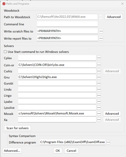
1. Download the HiGHS solver and save the executable in a subdirectory (e.g., C:\Solvers\HiGHS\highs.exe). In Woodstock, use Tools|Paths & programs to point to highs.exe in the GNU choice.
2. Create a text file called highs.par. Include the following line of code to specify the solution file format (GLPSOL): write_solution_style=3. If you're solving a MIP formulation, options like heuristics (%) and gap% are useful: mip_heuristic_effort=0.3 mip_rel_gap=0.001 
3. In Woodstock, specify *FORMAT GNU in the OPTIMIZE section. 
4. Press F9 to generate the matrix and create the batch file. You need to edit the batch file that Woodstock creates to comply with HiGHS command line parameters similar to below: C:\Solvers\Highs\highs.exe --model_file "model.mps" --solution_file "model.prt" --options_file highs.par
5. Use the Run|Run model.bat file menu or press F7 to call the solver and write the SCHEDULE section.

A Quirk of the HiGHS Solver

Although the programmable interfaces to HiGHS allow you to change the objective sense (MAX vs MIN), I didn't find any options in the command line interface to allow anything other than minimization. However, this is not a real problem because a MAX problem can be converted to a MIN problem by simply multiplying the outputs by -1. For example, the line 

            _MAX ordTOT - ocdLOG - ocdPLT 1..._LENGTH

can be converted to the equivalent statement 

           

            _MIN ocdLOG + ocdPLT - ordTOT 1.._LENGTH

Summary

If you are not running MIP formulations and you have MOSEK, there's nothing to see here folks. MOSEK is a very capable LP solver. Similarly, if you have access to Gurobi or CPLEX through school or corporate licensing, HiGHS is not going to be compelling. However, if you're interested in trying out some MIP formulations without investing a ton of money into a solver like Gurobi or CPLEX, give HiGHS a try. I'm hoping that Remsoft will soon support this new solver so that we don't have to do this messing around with batch files, etc. However, it is a small price to pay for a capable solver even now.

Don't hesitate to contact me if you have questions about this or other modeling topics!